The first thing that must be done when conducting data analysis is to form the collected data into a structure that is easy to analyze. Therefore, this section describes the data types and data structures used when analyzing data in R.
What are data types and data structures in R?
3 basic data types:
- Numeric
- Charactor
- Logic
5 basic data structures

- vector
- matrix
- array
- data frame
- facotr
- list
A solid understanding of these data types and data structures will be very helpful in understanding how R works in the future. This is a bit long article, but I will try to explain types and structures of r as clearly as possible.
Sample data creation
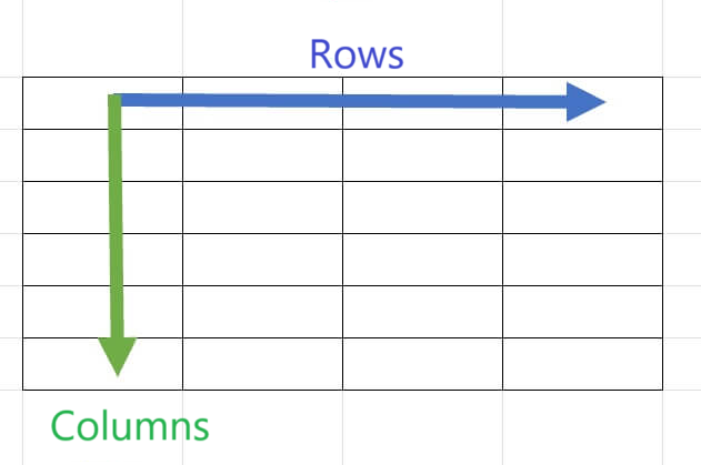
First, the data set (data you collect) is usually referred to as "rows" in the horizontal direction and "columns" in the vertical direction, with the rows representing observed values and the columns representing variables.

Let's generate imaginally COVID-19 test data below.
- Patient ID (ID)
- age (age)
- vaccination (with: T, without: F)
- type (alpha and beta strains)
- condition(mild, moderate, severe, critical).
| ID | age | vaccine | type | condition |
| 1 | 25 | F | alpha | severe |
| 2 | 34 | T | beta | mild |
| 3 | 28 | T | beta | moderate |
| 4 | 52 | F | alpha | moderate |
| 5 | 71 | T | alpha | critical |
The data structures like the sample data are called "data frames" in the R. Data frames can handle a wide variety of data types, giving you great flexibility in handling data in R. (This is explained in more detail in the later section.)
Data types handled by R
Let's take the data set above as an example to understand data types.
First, the scale of each data,
- ID, vaccine, type: nominal scale (ID is a nominal measure because it is a case identifier)
- age: ratio scale
- condition: ordinal scale
Here is a brief summary of the four primary levels of measurement.
A nominal scale is a scale for classifying data into categories, with no ordering or size information. Examples include blood type and gender.
An ordinal scale is a meaningful measure of the order, but the intervals between the orders are not constant. For example, rankings such as satisfaction and favorability are ordinal scales.
The interval scale is a scale where the data are spaced at a constant interval and the order is meaningful. However, there is no absolute zero point, so ratios cannot be determined. Temperature in degrees Celsius and IQ scores are examples of interval scales.
A ratio scale is a measure that has absolute zero points in addition to the order and spacing of the data. This makes it possible to determine the ratio of data. For example, height and weight are examples of ratio scales.
And R data types include numeric, character, and logical types. In the sample data above,
- ID, age:numeric
- vaccine:logical
- type, condition:charactor
R Data Type Basics
Numeric data is both integer and double.
For example,
x <- c(1, 4, 5, 10, 3)
y <- c(1.3, -10, 5, 6,11)
Character data deals with characters, which are enclosed in double quotation marks (" ").
For example,
x <- c("Tom", "Mike", "Ken")Boolean data is data that is handled as "true" or "false". It is also frequently used to analyze the logical type by replacing TRUE=1 and FALSE=0 with numbers.
For example,
y <- c(T,F,T,T)TRUE is abbreviated as T, FALSE as F.
Without abbreviation, you can type "Y <- c(TRUE,FALSE,TRUE,TRUE) ".
TRUE=1 and FALSE=0, so y can be summed,
sum(y)
[1] 3
then 3 will be returned.
How to check data types in R
In R, there are "typeof" function and "mode" function as a way to check data types. For example, using the example above, let's check the data type with the "typeof" function and the "mode" function.
Type of return value:
- "
typeof"function: Indicates the basic type of data based on the internal representation of the object. For example, "double" or "character" is returned. - "
mode" function: indicates the first class found among the available classes of objects. It expresses the data type in terms of higher-order concepts. For example, "numeric" or "character" is returned.
x <- c(1, 4, 5, 10, 3)
typeof(x)
[1] "double"

mode(x)
[1] "numeric"

y <- c(1.3, -10, 5, 6,11)
typeof(y)
[1] "double"

mode(y)
[1] "numeric"
In the example above, the typeof function returned "double" and the mode function returned "numeric".
Try the same for character types and boolean types.
x <- c("Tom", "Mike", "Ken")
typeof(x)
[1] "character"

mode(x)
[1] "character"

y <- c(T,F,T,T)
typeof(y)
[1] "logical"

mode(y)
[1] "logical"
Data structures handled in R
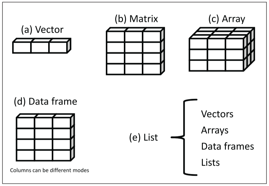
I mentioned at the beginning of this article that R has five data structures for holding data, such as vectors, matrices, arrays, data frames, and lists. The following figure shows each of these data structures.

Each data structure differs in terms of the type of data it can hold, how it is created, the complexity of its structure, and the notation used to identify and access individual elements.
vector
First, let's start with the most basic structure, "vector".
A vector is a one-dimensional array that can store just one of the following types of data: numeric, character, or logical type data. To form a vector, use the c() function.
For example,
x <- c(1, 2, 3,4,5)

y <- c("one", "two", "three", "four", "five")

z <- c(T, T, F, T, F)
In the example above, x is a numeric type vector, y is a character type vector, and z is a logical type vector.
The most important point here is that a vector can contain one type (either numeric, character, or logical type) of data. As in the example below, you cannot mix different forms of data in a vector.
a <- c(1, 2, "one", "two", T, F)If you run the code above, you will see everything is forced to be converted to Character type.
print(a)
[1] "1"     "2"     "one"   "two"   "TRUE"  "FALSE"
How to check elements in a vector
If the data is small, as in the example above, you can see the elements in a vector just by looking at the data, but in a research or survey, a single vector may contain more than 1000 or even more datas. Then it is difficult to visually find certain values among these huge amounts of data. In such cases, an index ([ ]: square brackets) is used to refer to any numbered vector element.
x <- c(1, 2, 3, 4, 5)
x[2] #extract second element

[1] 2
"2" which is the second element of x is returned.
You can also specify consecutive numbers by using the colon (:) operator. In the case below, elements can be retrieved by the second through fourth elements.
x[2:4] #Extract the 2nd through 4th elements

[1] 2 3 4
matrix
A matrix is a two-dimensional array in which each element has the same data type (numeric, character, or logical). Matrices are created using the "matrix" function.
The general matrix format is as follows
x <- matrix(vector, nrow=number_of_rows, ncol=number_of_columns, byrow=T or F, dimnames=list(char_vector_rownnams, char_vector_colnames)))
- vector: vector (or data)
- nrow/ncol : Abbreviation for number of rows and number of columns. Specifies the dimensions of rows and columns. In other words, "horizontal and vertical" matrices are specified.
- byrow: Specifies how the vectors (data) are arranged:
- If data is arranged by row, byrow=TRUE
- If the data is to be sorted by column, byrow=FALSE (the default is by column).
- dimnames :Set row and column names
As an example, let's create a 5X4 matrix.
First, when arranged by row,
rnames<-c("R1", "R2", "R3", "R4", "R5")
cnames<-c("C1", "C2", "C3", "C4")

x <- matrix(1:20, nrow = 5, ncol = 4, byrow = TRUE, dimnames = list(rnames, cnames))

x
   C1 C2 C3 C4
R1  1  2  3  4
R2  5  6  7  8
R3  9 10 11 12
R4 13 14 15 16
R5 17 18 19 20
Next, when arranged by columns,
y <- matrix(1:20, nrow = 5, ncol = 4, byrow = FALSE, dimnames = list(rnames, cnames))

y
   C1 C2 C3 C4
R1  1  6 11 16
R2  2  7 12 17
R3  3  8 13 18
R4  4  9 14 19
R5  5 10 15 20
Think of a matrix as a vector with a two-dimensional structure. Therefore, like a vector, it can only contain one data type. If the data structure exceeds two dimensions, use array as described below. If there are multiple data types, use data frames instead of matrices.
Extract the elements in the matrix
Like vectors, the index ([ ]: square brackets) can be used to identify the row and column elements of a matrix.
X[i,] means the element in "row i" of matrix X, X[,j] means "column j", and X[i, j] means "column j of row i", respectively.
Selecting multiple rows or columns is easy with a colon (:) or c( ).
For example, the following matrix can be used to extract elements by specifying rows, columns, and rows x columns.
x <- matrix(1:10, nrow=2)

x
     [,1] [,2] [,3] [,4] [,5]
[1,]    1    3    5    7    9
[2,]    2    4    6    8   10
x[2,] #Select all elements on the second line
[1] 2 4 6 8 10x[,2] #Select all of column 2
[1] 3 4x[1,4] #Select elements in row 1 x column 4
[1] 7x[1, c(4,5)] #Select elements in row 1 x columns 4 and 5
[1] 7 9array
Arrays are similar to matrices, but they can have a multi-dimensional data form with more than two dimensions.
The array uses the "array function" and the general form is as follows
x <- array(vector, dimensions, dimnames)
- vector : vector (or data)
- dimensions : The number of dimensions in each dimension of the array. For example, c(2, 3, 4) would be four 2x3 matrices
- dimnames : Name of each dimension
As an example, let's create a 3-dimensional (2x3x4) array as follows.
dim1 <- c("X1", "X2")
dim2 <- c("Y1", "Y2", "Y3")
dim3 <- c("Z1", "Z2", "Z3", "Z4")
z <- array(1:24, c(2, 3, 4), dimnames=list(dim1, dim2, dim3))
z
, , Z1
Y1 Y2 Y3
X1 1 3 5
X2 2 4 6
, , Z2
Y1 Y2 Y3
X1 7 9 11
X2 8 10 12
, , Z3
Y1 Y2 Y3
X1 13 15 17
X2 14 16 18
, , Z4
Y1 Y2 Y3
X1 19 21 23
X2 20 22 24Thus, it is easier to understand arrays by thinking of them as an extension of matrices. Like vectors and matrices, arrays can only store one type of data.
Keep in minds, the more multidimensional it becomes, the more difficult it becomes to visualize.
data frame
Unlike previous data types, data frames are the most important data type in data analysis in that they can contain multiple types of data (numeric, textual, ethical, etc.). In addition, data frames are the most common data structure handled in R because they are the closest form to the data sets collected in Excel and other applications.
Data frames are created with the "data.frame" function and the general form is as follows
x <- data.frame(col1, col2, col3,...)
- col1, col2, col3, … is the data contained in each column.
As an example, let's create a data frame of the imaginally COVID-19 test data shown at the beginning of this section.
| ID | age | vaccine | type | condition |
| 1 | 25 | F | alpha | severe |
| 2 | 34 | T | beta | mild |
| 3 | 28 | T | beta | moderate |
| 4 | 52 | F | alpha | moderate |
| 5 | 71 | T | alpha | critical |
ID <- c(1, 2, 3, 4, 5)
age <- c(25, 34, 28, 52, 71)
vaccine <- c(F, T, T, F, T)
type <- c("alpha", "beta", "beta", "alpha", "alpha")
condition <- c("severe", "mild", "moderate", "moderate", "critical")

pt_data <- data.frame(ID, age, vaccine, type, condition)
pt_data
ID age vaccine type condition
1 1 25 FALSE alpha severe
2 2 34 TRUE beta mild
3 3 28 TRUE beta moderate
4 4 52 FALSE alpha moderate
5 5 71 TRUE alpha criticalIn a data frame, there must be one data type within each column, but different columns can consist of different data types.
If you check, you will see that the data frame is composed of different data types.
> typeof(pt_data$ID)
[1] "double"
> typeof(pt_data$age)
[1] "double"
> typeof(pt_data$vaccine)
[1] "logical"
> typeof(pt_data$type)
[1] "character"
> typeof(pt_data$condition)
[1] "character"
Extract elements in a data frame
There are several ways to extract elements from data frame.
- Use index ([ ]: square brackets)
- Use dollar sign ($)
By index ([ ]: square brackets)
As with the method described in the vector and matrix sections, elements can be retrieved by specifying column names in the index ([ ]: square brackets). For example, to retrieve the elements of "ID" and "age" of pt_data created, just specify the column number.
pt_data[1:2] #Extract elements in columns 1 and 2

  ID age
1  1  25
2  2  34
3  3  28
4  4  52
5  5  71
The elements from "ID" and "age" can be extracted.
You can also specify column names instead of column numbers. For example, if you want to extract the "type" and "condition" elements of pt_data, use [ ] and c( ) to specify column names.
pt_data[c("type", "condition")] #extract elements of type and condition columns

   type condition
1 alpha    severe
2  beta      mild
3  beta    moderate
4 alpha   moderate
5 alpha   critical
If you want to retrieve more specific values,
> pt_data[2,4]
[1] "beta"
then the elements of the second row x fourth column can be extracted.
By $ (dollar sign)
The $ symbol is frequently used to specify a specific column from a data frame. For example, if you specify the "age" of pt_data,
pt_data$age
[1] 25 34 28 52 71
The data of "age" can be retrieved.
You can easily create a cross-table by using the following "table" function with "$".
table(pt_data$type, pt_data$condition) critical mild moderate severe
alpha 1 0 1 1
beta 0 1 1 0factor
Nominal and ordinal scale variables are qualitative (categorical) data and have no distinct order. Using the pt_data example above, type (alpha, beta) is an example of a nominal scale. Even though alpha is coded as 1 and beta as 2 in the data, the order is not clear. Also, conditon (mild, moderate, severe, critical) is an ordinal scale variable, meaning order without a clear interval. So we know that SEVERE is in "worse condition" than MILD or MODERATE, but we don't know how much difference there is between each.
For such qualitative (categorical) data, R uses factor.
Factor uses the "factor" function to replace category values with a vector of integers and store the original values mapped to these integers. For example,
type <- c("alpha", "beta", "beta", "alpha", "alpha")
type <- factor(type)

type
[1] alpha beta beta alpha alpha
Levels: alpha beta
Then the values above are assigned internally with alpha=1 and beta=2. In the example above, "alpha beta beta alpha alpha" is "1 2 2 1 1 1".
The default order of this assignment is alphabetical.
condition <- c("severe", "mild", "moderate", "moderate", "critical")
condition <- factor(condition)

condition
[1] severe mild moderate moderate critical
Levels: critical mild moderate severe
then the data vector in condition is replaced as (4 2 3 3 1) and these values are internally associated with critical=1, mild=2, moderate=3, and severe=4.
This alphabetical order may cause confusion in data interpretation. In the case of an example above, it's easier to interpret if the better the condition, the smaller the number. In this case, add the optional LEVELS like below.
condition <- factor(condition, order=TRUE, levels=c("mild", "moderate", "severe", "critical"))

condition
[1] severe mild moderate moderate critical
Levels: mild < moderate < severe < critical
This way, the levels are assigned as follows: mild=1, moderate=2, severe=3, critical=4, and so on!
List
List is the most complex of R's data structures. It allows you to freely arrange various types of data in a single list.
The general form of "list" function is following .
x <- list(object1, object2, ...)
Let's create a list to try it out.
x1 <- "My favorite things"
x2 <- c(1, 2, 3, 4, 5)
x3 <- matrix(1:10, nrow=5)
x4 <- c("TOM", "KEN", "JOE")
x <- list(text=x1, x2, x3, friend=x4)
x
$text
[1] "My favorite things"
[[2]]
[1] 1 2 3 4 5
[[3]]
[,1] [,2]
[1,] 1 6
[2,] 2 7
[3,] 3 8
[4,] 4 9
[5,] 5 10
$friend
[1] "TOM" "KEN" "JOE"You can name each list. You can see that list items with names(text and friend) are marked with a $ sign, and lists without names are marked with [[list number]]. You can use this $ and [[ ]] to specify the elements of a list.
x$text
[1] "My favorite things"

x[[2]]
[1] 1 2 3 4 5
summary

In this article, I explained the data types and data structures handled in R with examples so that even beginners can understand them.


コメント