Classification of Variables
In this article, we'll introduce key concepts in descriptive statistics, starting with how to classify different types of variables and visualize them using histograms.
Variables

We will begin by discussing how to classify variables.
In statistics, variables are the main objects of analysis, so let’s first organize the different types of variables.
To help understand what a variable is, I’ve prepared an example table with sample data.
| State | Average Temperature (°F) | Population (in millions) |
| California | 65 | 39.5 |
| Texas | 70 | 29.0 |
| Florida | 75 | 21.5 |
| New York | 55 | 19.5 |
| Illinois | 52 | 12.5 |
| Pennsylvania | 50 | 12.8 |
| Ohio | 51 | 11.7 |
| Georgia | 68 | 10.7 |
In this table, the rows (which we call the "stub") represent the states of the United States.
The columns (called the "head") list state names, average temperature, and population.
So, what are the variables in this table?
In the table, each column represents a variable — for example, "State Name," "Average Temperature," and "Population."
Classification of variables
Now, we’d like to organize and classify these variables.
Variables can be categorized according to four types of measurement scales.
You can think of these scales like measuring tools for data.
The four scales are: nominal, ordinal, interval, and ratio scales.
Nominal Scale:
Let’s begin with the nominal scale.
This scale is used where the only meaningful distinction is whether values are the same or different.
Examples include gender (male/female), or occupation (company employee or self-employed).
There is no inherent order or ranking between the values.
Ordinal Scale:
Next is the ordinal scale, where not only sameness or difference is meaningful, but also the order of the values.
For instance, evaluation ranks like A, B, C have an order.
Levels of satisfaction like "dissatisfied, neutral, satisfied" also have a meaningful sequence.
Interval Scale:
Going further, when the difference between values is also meaningful, we call this the interval scale.
A good example is temperature.
The difference between 10 and 11 degrees has the same meaning as the difference between 11 and 12 degrees.
Since the intervals are uniform and meaningful, temperature is considered an interval-scale variable.
Ratio Scale:
Lastly, the ratio scale includes variables where not just the order and interval,
but also the ratios between values carry meaning.
That is, these variables have a true zero point, and we can interpret values proportionally based on that zero.
Examples include length, weight, and price.
For example, 10 cm is twice as long as 5 cm, and $200 is double the price of $100.
By contrast, with interval variables like temperature, we don’t say "20 degrees Fahrenheit is twice as hot as 10 degrees Fahrenheit"—because zero does not represent a true absence of temperature.
This ability to express proportional relationships is the key difference between interval and ratio scales.
So, to summarize the four types of scales:
- Nominal scale and ordinal scale variables are called qualitative variables. These are more like labels or tags rather than things that can be measured with a ruler.
- Interval scale and ratio scale variables are called quantitative variables. These are measured with a scale or ruler—real measurements.
- Interval scale variables use a ruler with evenly spaced units.
- Ratio scale variables use that same ruler but with a true zero, allowing for ratios to be interpreted.
Classification of Variables
| Category | Scale Type | Description | Examples |
| Qualitative | Nominal Scale | Categories with no natural order | Gender (Male/Female), Blood Type (A/B/O) |
| Ordinal Scale | Categories with a meaningful order, but not evenly spaced | Grades (Excellent/Good/Fair), Satisfaction (High/Medium/Low) | |
| Quantitative | Interval Scale | Numeric values with equal intervals, but no true zero | Temperature (°F), Calendar Years (e.g., 1990) |
| Ratio Scale | Numeric values with equal intervals, and a meaningful zero, allowing ratio | Height, Weight, Population |
Next, we’ll move on to histograms—a tool used to visualize the distribution of quantitative variables we've just discussed.
Histograms and Cumulative Distributions (Quantitative Variables)
Let’s look at histograms and cumulative distributions.
Histograms and cumulative distributions are graphs used to understand how frequently certain values of a quantitative variable occur—in other words, to understand the distribution of a variable.
To draw a histogram or cumulative distribution, we use something called a “frequency distribution table”, as shown below.
| Age Group | Frequency (in millions) | Relative Frequency (%) | Cumulative Relative Frequency (%) |
| Under 10 | 8.0 | 9.64 | 9.64 |
| 10–19 | 8.5 | 10.24 | 19.88 |
| 20–29 | 7.0 | 8.43 | 28.31 |
| 30–39 | 10.0 | 12.05 | 40.36 |
| 40–49 | 11.0 | 13.25 | 53.61 |
| 50–59 | 12.0 | 14.46 | 68.07 |
| 60–69 | 11.0 | 13.25 | 81.33 |
| 70–79 | 9.0 | 10.84 | 92.17 |
| 80 and over | 5.5 | 6.63 | 98.80 |
| Unknown/Other | 1.0 | 1.20 | 100.00 |
It's a bit complicated, so please be careful. In this case, we have a quantitative variable called "age," which we divide into classes. We then count the frequency for each class.
So, what we have is a frequency distribution table for the variable "age."
To read the table, we can interpret it like this—the count for the under-10s is 8 million, the count for the 20s is 7 million, and so on.
So, what would the histogram for this frequency distribution table look like? It would look like this.
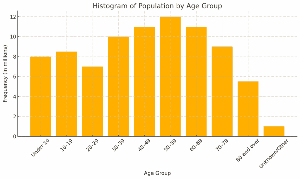
One important point when drawing a histogram is that since we're examining the distribution of a variable, we place the variable on the horizontal axis and the frequency distribution (count for each class) on the vertical axis.
In this histogram, the horizontal axis represents the variable "age," while the vertical axis shows the frequency of each age group.
This histogram provides a clear visual of how the population is distributed across different age groups.
Cumulative Distribution
While a histogram shows how frequently each value or group occurs, a cumulative distribution shows how data adds up over time or across categories. It helps you understand "how much so far". In other words, instead of looking at each group separately (like histogram), cumulative distribution adds up the values step by step.
It shows growth or accumulation over time or steps. It's also easy to see milestones, like when you've reached 50% or 80% of the total.
To draw a cumulative distribution, we need something called relative frequency.
Relative frequency is calculated by taking the total frequency — regarded as 100% and determining the proportion each class contributes to that total.
For example, if the count for the under-10s is 8 million, then the relative frequency is 9.64%. We can draw the relative frequency graph as shown below.

By accumulating (adding up) the relative frequencies in order from the smallest class upward, we get the cumulative relative frequency. Using this, we can draw the cumulative distribution graph.
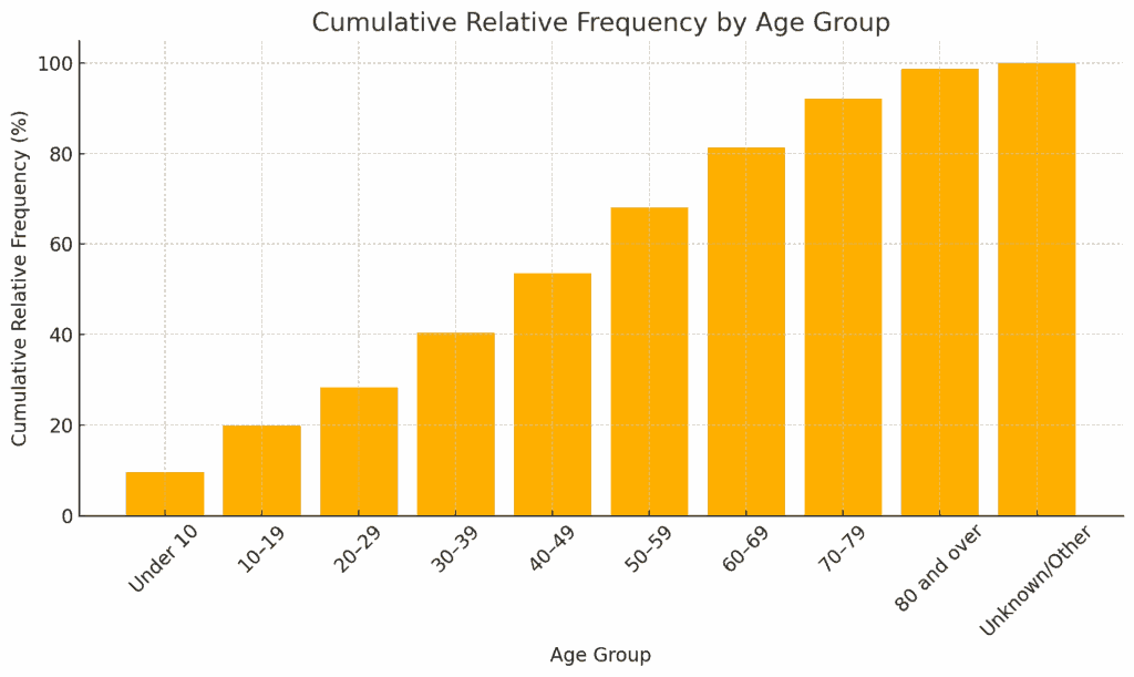
Now, what does the cumulative distribution graph look like? It looks like this. The horizontal axis is again the variable "age," and the vertical axis shows the cumulative relative frequency from the frequency distribution table.
While the histogram shows each class individually, the cumulative distribution graph lets us check the cumulative relative frequency up to each class.
For example, when the cumulative relative frequency reaches 50%, it falls somewhere between the 40–49 age group. This indicates that about half of the population is aged below 50.
Conclusion:

In this article, we explored the foundations of descriptive statistics—starting with how to classify variables and moving on to tools like histograms and cumulative distributions.
Understanding the types of variables helps us choose the right methods to analyze them, while frequency tables and visualizations like histograms allow us to see patterns in the data more clearly. Cumulative distributions take this a step further by showing how values accumulate over a range.
These are essential building blocks for anyone beginning to study data!


コメント